Muscle preparations

            We have been employing skinned single muscle fibers for our research. Its plasma membrane is functionally removed by a chemical treatment so that experimenters can access contractile proteins directly from outside: one can apply desirable solutions to test a particular hypothesis. Advantages of this preparation is (1) contractile proteins are structured and in high concentration, so that the cooperativity between proteins is present as it occurs in muscle cells, (2) physiological solutions that mimic in-situ concentrations in myoplasm can be applied so that the results are readily applicable to the physiological conditions. Disadvantages are that the skinned fiber is still a complex system, and a very clever method must be developed to sort out the results. Both (1) and (2) are absent in the in-vitro systems, which are serious disadvantages.

            Rabbit psoas single fibers that are chemically skinned are our typical preparations (Fig. 1B); we have also used other rabbit skeletal muscle fibers (EDL, semitendinosus, soleus, etc). We have also used skeletal muscle fibers from crayfish walking leg, frog semitendinosus, and compared results from intact vs. skinned fiber preparations. Furthermore, we have used heart muscle strips of cows, pigs, rabbits, rats and mice. For heart muscles, we selectively removed the thin filament by gelsolin treatment, and reconstituted the thin filament with constituent proteins. The thin filament reconstituted preparations are convenient to study the structure-function relationship of contractile proteins, and genetically altered mutant proteins that cause cardiomyopathy. 

Sinusoidal Analysis 

      The sinusoidal analysis method can be described as follows. If you tap a wooden table, you hear a sound (resonance) that suggests wood. If you tap a steel table, you hear a sound that suggests steel. By tapping the muscle fibers (meaning change in their length in various speed, or frequency), you hear a resonance from a chemical reaction that takes place in the muscle. To generate the resonance, the chemical reaction must be mechanically coupled to a change in the strain (length), else no resonance will be generated. By changing the frequency, you hear resonances from different chemical reactions.

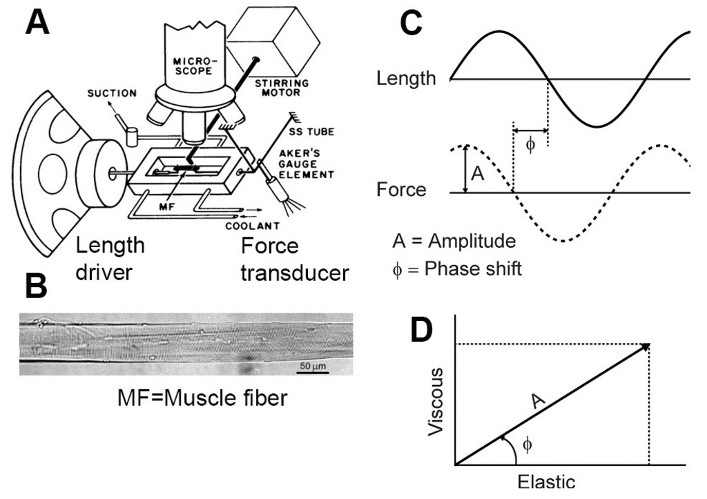
Figure 1

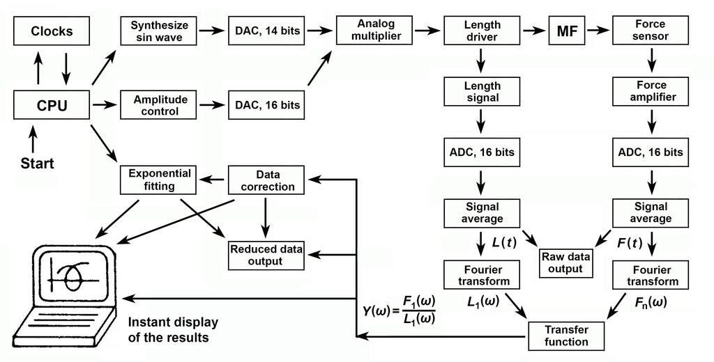
Figure 2

        A skinned muscle fiber (MF, Fig. 1A & B) is mounted horizontally in the experimental chamber (Fig. 1A). The length of the fiber is changed in a sinewave with a frequency f (Fig. 1C) that is digitally synthesized, and concomitant force time course is collected. The information we extract is the amplitude and the phase shift (Fig. 1C) from force time course. The amplitude of force change is divided by the amplitude of the length change, and normalized to the size of the preparation. The result is called “Complex modulus, Y(f)”. This is plotted on the polar coordinate as a vector (arrow in Fig. 1D): the phase shift as its angle (ϕ) from X-axis, and the amplitude (A) as the length of the vector. Its X-projection is called the Elastic modulus (EM), and Y-projection is called the Viscous modulus (VM). This type of plot is called "Nyquist plot". In the complex plane, EM is the real part, and VM is the imaginary part of the complex number Y(f). 

        EM represents how stiff the muscle is. With EM, the preparation absorbs work when stretched, and releases the same amount of work when shortened: the net work is 0. A spring is a good example of EM. VM represents the amount of work absorbed by the preparation: when VM is positive, muscle absorbs work from the forcing apparatus (length driver) both during stretch and release. This work is lost as the heat. Friction is a good example of VM. When VM is negative, muscle generates work on the forcing apparatus. This property is called "oscillatory work" because muscle performs work on oscillating length driver. This work comes out from ATP hydrolysis. The complex modulus Y(f) is studied as functions of frequency (f) in the range 0.25Hz and 250Hz in fast twitch muscle fibers. Fig. 2 is a flow chart of these operations performed under the computer control by a home made program DCOLL.exe.

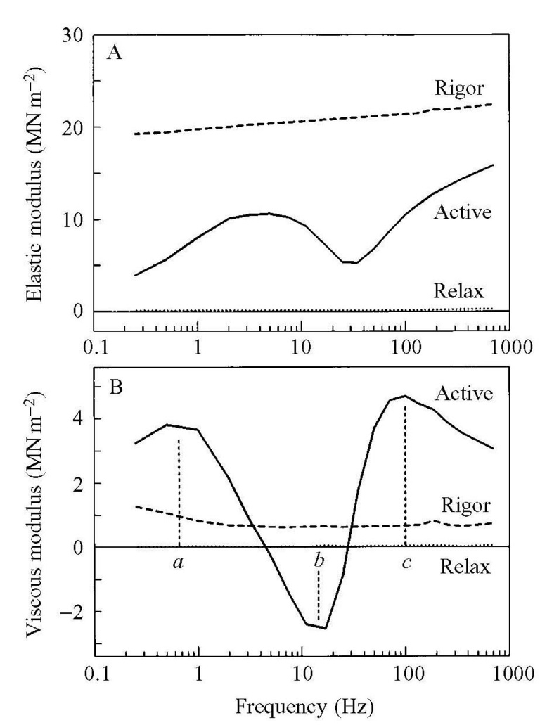
                                             Figure 3

        Fig. 3A plots EM, and Fig. 3B VM of rabbit psoas fibers against frequency (f) at three conditions (Active, Rigor, and Relaxation). Muscle in rigor is very stiff, and it behaves like a spring: EM is large, VM is small, and they do not change much with the frequency. When the muscle is relaxed, both EM and VM are very small, indicating that the length change is not much registered as force change, as if no preparations are in place. When the muscle is activated, two plots have more complex and interesting features as shown in Fig. 3. The VM has two absorption peaks (a and c), and one negative peak (b) with a<b<c; these are called characteristic frequencies, and if multiplied by 2π, they represent the apparent (=measured) rate constants. The EM during activation at low frequencies (such as ≤0.5Hz) is small, because cross-bridges have enough time to adjust to the imposed length change. The EM is large at high frequency (such as ≥250Hz), because the cross-bridges do not have enough time to adjust to the imposed length change. In the middle frequency range (10-100Hz), length change and the cross-bridge cycle beat each other to have a complex plot as shown in Fig. 3. In the Nyquist plot, the data from active fiber  result in a bifoliate shape as shown in Fig. 4A.

        By analyzing the bifoliate shape, we have been able to deduce the molecular mechanisms of the cross-bridge cycle. Our investigations have demonstrated that the characteristic frequency c represents the rapid cross-bridge detachment step after ATP binding; frequency b represents the cross-bridge attachment and force generation steps; and frequency a represents the step that generates the work. The force generation and work production are two different steps. 

        The complex modulus data are satisfactorily explained by Eq. 1:

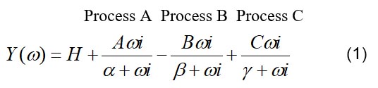
where ω=2πf, α=2πa, β=2πb and γ=2πc are apparent (measured) rate constants (0<a<b<c). A, B and C (all positive numbers) are their respective magnitudes (amplitudes); H is a constant. Note the negative sign for process B in Eq. 1. Each process is called “exponential process”, because its time domain expression consists of an exponential function (Eq. 2):

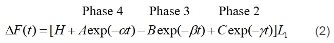
where L₁ is the step size; L₁>0 for stretch, and L₁<0 for release.  “Phases” are the phases of force response in response to a step length change, and different from phase shit of the sinusoidal analysis. It is clear from Eqs. 1 and 2 that process A corresponds to phase 4, process B to phase 3, and process C to phase 2; Y_∞ corresponds to phase 1, where     

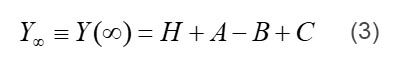
             Fig. 4 shows the correlation between exponential processes of sinusoidal analysis (Fig. 4A), and phases of step analysis (Fig. 4B). They are related by a linear transformation (LT–LT’ with slope L₁) in Fig. 4A and B. In Fig. 4B, a step increase in length takes place at t=1 ms, and tension time course is plotted in the log time axis. Fig. 4C represents the mechanical equivalence of the complex modulus response by active fast twitch muscle fibers. Here the process B (oscillatory work) is represented by intertwined two rings. 

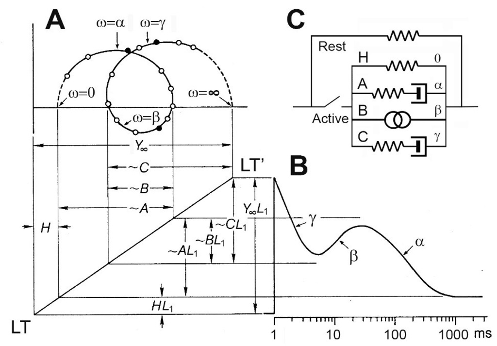
Figure 4

ATP and ADP effects, and cross-bridge detachment step

To study the elementary steps (K₁, k₂, k_-2) surrounding the ATP binding step 1, the S=[ATP] is changed such as 0.1, 0.2, 0.5, 1, 2, 5, 10 mM, and the apparent rate constant 2πc is studied. The result is plotted in Fig. 5A.

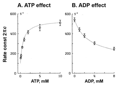
Figure 5

2πc increases at 0.1-2 mM ATP, and then approaches saturation, exhibiting a typical hyperbolic curve. Such result can be explained by steps 1 and 2 of scheme 1. 

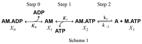
where K₁=ATP association constant (step 1), k₂=the rate constant of cross-bridge detachment (step 2) which ensue the ATP binding, and k_-2=the rate constant of its reversal step. For the ATP study, the step 0 is absent. Eq. 4 relates the kinetic constants (K₁, k₂, k_-2) and the ATP concentration (S) to the apparent rate constant 2πc:

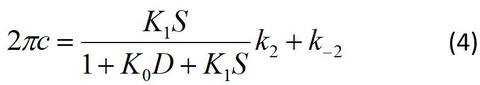
By fitting the data to Eq. 4, one can deduce three kinetic constants K₁, k₂, and k_-2. Here D=[ADP] is assumed to be 0, because there is practically no ADP in the presence of the ATP regenerating system (phosphocreatine and creatine kinase with Lohman reaction). The data fits well as shown in the continuous curve in Fig. 5A, demonstrating the high credibility of the model shown in Scheme 1. Here it is important to note that we do not deduce unnecessarily many (>3) parameters from the data, and Scheme 1 with steps 1 and 2 is the minimal model to account for the data. If one deduces more parameters in an attempt to explain more complex model than Scheme 1, the credibility of the model becomes thin and its significance gets lost. K₂ is calculated as K₂=k₂/k_-2, hence this is not an independent parameter.

                To study the elementary step 0, ADP concentration (D) is changed such as 0, 1, 2, 4, 8 mM (in the absence of the ATP regenerating system), and the apparent rate constant 2πc is studied (Fig. 5B) at constant [ATP] (5 mM). The result is a decreasing hyperbolic function, and such curve is fitted to Eq. 4, where we use K₁ obtained from the ATP study and deduce only one parameter K₀, the ADP association constant. The data fits well as shown in the continuous curve in Fig. 5B.

Phosphate effect, and the force-generation step

To study the elementary steps (k₄, k_-4, K₅) surrounding force generation and the phosphate (Pi) release steps, P=[Pi]=[phosphate] is changed such as 0, 2, 4, 8, 16 mM at a constant ATP concentration (5 mM), and the apparent rate constant 2πb is studied.

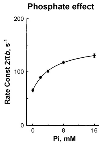
Figure 6

The result is plotted in Fig. 6. 2πb increases at low mM of Pi, and then approaches saturation, exhibiting a typical hyperbolic saturation curve. Such result can be explained by steps 4 and 5 of scheme 2.

Scheme 2

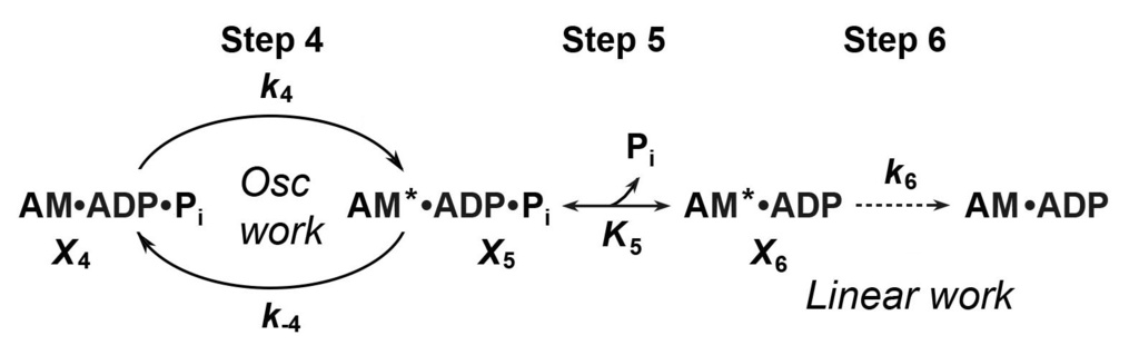
where k₄=the rate constant of the force generation step 4, k_-4=its reversal step, and K₅=Pi association constant. AM.ADP.Pi is the weakly attached state, which is in rapid equilibrium with the truly detached state (M.ADP.Pi) with the equilibrium much to the detached state, hence AM.ADP.Pi is present only briefly (transiently). For this reason, step 4 is often called the "cross-bridge attachment step". Force is generated in step 4, hence AM*ADP.Pi is the strongly attached state, and the same force is maintained with Pi release (step 5). 

Eq. 5 relates the kinetic constants (k₄, k_-4, K₅) and the Pi concentration (P) to the apparent rate constant 2πb:

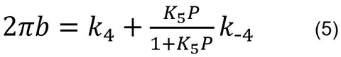
By fitting the data to Eq. 5, one can deduce three kinetic constants k₄, k_-4, and K₅. The data fits well as shown in the continuous curve in Fig. 6, demonstrating the high credibility of the model shown in Scheme 2. Here it is important to note that we do not deduce unnecessarily many (>3) parameters from the data, and Scheme 2 with steps 4 and 5 is the minimal model to account for the data. If one deduces more parameters in an attempt to explain more complex model than Scheme 2, the credibility of the model becomes thin and its significance gets lost. K₄ is calculated as K₄=k₄/k_-4, hence this is not an independent parameter.

            As shown in Scheme 2, cyclic reactions within step 4 constitutes the oscillatory work. Step 6 is the slowest step in the cross-bridge cycle, hence it limits the ATP hydrolysis rate. It is mostly unidirectional. Because force is generated at step 4, the cross-bridge is ready to perform work (such as lifting load) both at steps 5 and 6.  Because lifting the load takes time, the most work is done on step 6 (much slower than step 5). This is commented as “linear work” in Scheme 2.

Cross-bridge distribution and the force/cross-bridge state

Now let’s define that X₄, X₅, X₆ represent the probability of cross-bridges in states AM.ADP.Pi, AM*ADP.Pi, AM*ADP, respectively, as correlated in Scheme 2. That is: if X’s are multiplied by the total myosin head (S1) concentration, then the result is the concentration of each molecular species. Because the step 6 is the slowest step of the cross-bridge cycle, we can approximate by assuming that the step 6 does not happen in the time frame (speed) we observe the faster steps 4 and 5. This assumption sets up an equilibrium between the states X₄, X₅, X₆, and they can be readily solved.

               X₄=K₅P/M                 (6)

               X₅=K₄K₅P/M              (7)

               X₆=K₄/M                     (8)

where  M=  K₄+(1+K₄)K₅P       (9)

And            X₄+X₅+X₆=1           (10)

Now let’s assume that the force each cross-bridge state (X_j) carries (or supports) is T_j (j=4,5,6). Because cross-bridges are in parallel in each half sarcomere, the total tension (Ten) is:

Ten = T₄X₄ + T₅X₅ + T₆X₆ = T₅X₅ + T₆X₆    (11)

The term associated with X₄ is dropped, because it is the weakly attached or detached state, which does not carry or support force (T₄=0). By substituting Eqs. 6-10 in Eq. 11, we obtain Eq. 12:

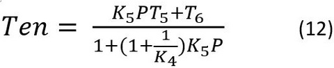
Eq. 12 hyperbolic decreasing function with P: it is T₆ at P → 0, and saturates at T₅K₄/(1+K₄) as P becomes large (P → ∞). K₄ and K₅ are obtained from the P dependence of the apparent rate constant 2πb (Eq. 5, Fig. 6). 

Fig. 7 plots Pi dependence of tension under two conditions (±Nebulin) in mouse soleus slow twitch fibers. Symbols are the observed tension , and continuous lines are best fit to Eq. 12. The thick line is based on the assumption that tension develops on step 4 (T₅>0) with isomerizarion, and the same force is maintained (T₆=T₅) with the Pi release (step 5), whereas the thin line (with #) is based on the assumption that tension develops on step 5 with Pi release, i.e., T₅=0 and T₆>0. They merge in the absence of Pi, because there is no AM*ADP.Pi state when P → 0. Fig. 7 is a good demonstration that tension is generated on step 4, and the same tension is maintained with Pi release. Fig. 7 also demonstrates that T₅=0 is a wrong assumption, i.e., tension does not develop with the Pi release. In practice, the Pi dependence of tension can be fitted to Eq. 12 to find T₅ and T₆ independently (this is a linear fitting, because Eq. 12 is linear to T₅ and T₆, although Eq. 12 is not linear to P). This fitting demonstrates that T₅≈T₆ >0. 

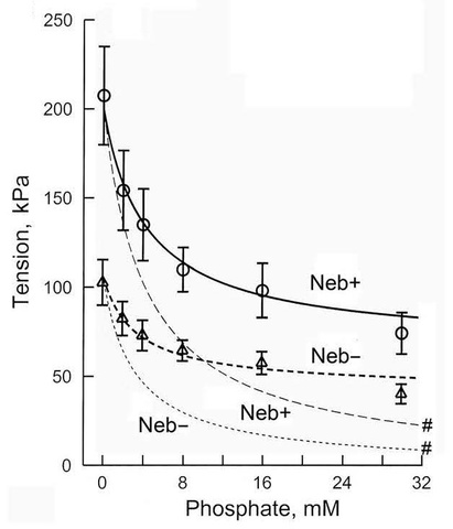
Figure 7

Eqs. 6-12 can be generalized to include both schemes 1 and 2 with six cross-bridge states. The probability of cross-bridges among these states is plotted in Fig. 8 under the two conditions (±Nebulin) in mouse soleus slow twitch fibers, activated at S=5 mM, P=8 mM, and D=0.01 mM with CP/CPK. Det=X₃₄=X₃+X₄, and the summation of weakly attached and detached states. Att=X₅+X₆+X₀+X₁+X₂=1-X₃₄ and the summation of all strongly attached states that are force-generating and/or force bearing states.

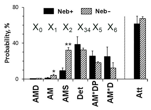
Figure 8

Fig. 9 plots tension generated or supported by each cross-bridge state for rabbit psoas fast twitch fibers, and soleus slow twitch fibers. As this plot shows, tension is generated at step 4, and same tension is maintained with Pi release step 5, ADP isomerization step 6, ADP release step 0; tension becomes about half after ATP binding followed by cross-bridge detachment from actin (step 2) in fast and slow twitch muscle fibers.

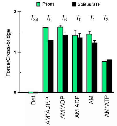
Figure 9

As demonstrated in Fig. 9, there is no evidence of extra force generation on ADP release (step 0) when measured under the physiological conditions both in fast twitch and slow twitch muscle fibers. 

Steps that generate work, and energy usage

  Once force is generated on a cross-bridge in the step 4 (AM*ADP.Pi), the muscle is ready to perform work, such as lifting a load. Thus work can be performed at any of steps 5, 6, 0 and 1. However, lifting a load takes time (τ). Step 5 (Pi release), step 0 (ADP release), and step 1 (ATP binding) are diffusion limited and fast, therefore, there is little time to perform work. In contrast, the step 6 is a slow reaction, hence suitable to perform work.

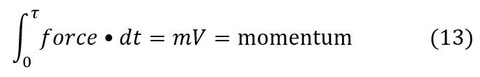
Here force-time integral is converted to the momentum of the motion (primarily at step 6), where m=mass of the load, and V=velocity of the movement, and τ=time the force is applied to the load. Consequently, we conclude that the step 6 (isomerization of ADP bound state) is the major work performance step. This is the "linear work", and all three quantities (force, velocity, momentum) in Eq. 13 have the same direction, hence they can be conveniently expressed by vectors. In contrast, the kinetic energy E_k transferred is:

                                               E_k = ½mV²                                        (14)

and this quantity does not have the direction.  Both momentum and the kinetic energy determine the movement of the load (V). 

  Because step 6 is the slowest step of the cross-bridge cycle, 

ATPase = k₆(AM*ADP) ‒ k_-6(AM.ADP) ≈ k₆(AM*ADP)   (15)

Thus, the rate constant of step 6 (k₆) is determined from the ATP hydrolysis rate on muscle fibers. The approximation of Eq. 15 (after ≈) is valid, because (AM*ADP) >> (AM.ADP) (Fig. 7) in the presence of the ATP regenerating system. (AM*ADP) is determined from Eq. 8. It is also known that k₆ >> k_-6 in the solution studies. Some investigators state that the ADP release step is slow: this is because steps 6 and 0 are frequently combined, hence the combined reaction appears slow.

  The efficiency of linear work performance Eff_Lin is:

                                             Eff_Lin = E_k/ATPase                            (16)

Cross-bridge cycle

Scheme 3 is the result of combining schemes 1 and 2. Scheme 3 also includes the ATP cleavage step 3 and the cross-bridge attachment step 3a to result in the AM.ADP.Pi state. The reactions during detached states are next to impossible to detect by mechanical measurements which depend on strongly attached states with a significant amount of lifetime. The strongly attached, but no-force generating state AM.ADP.Pi is a conceptual state, because otherwise force generation to result in the  AM*ADP.Pi (force bearing state) is not possible.

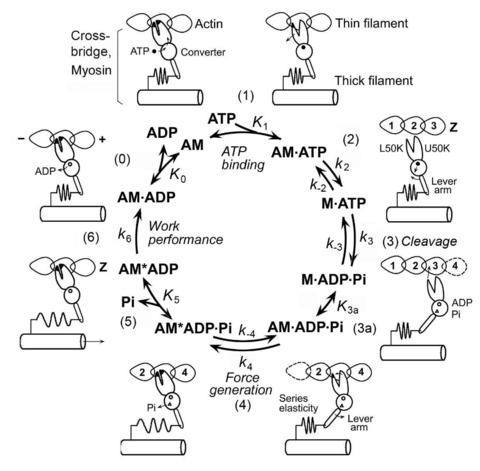
Scheme 3        

As described above, the kinetic constants (rate constants and equilibrium constants) of scheme 3 can be measured by sinusoidal analysis methods when concentration effects of ATP, Pi, and ATP (S, P, D, respectively) on the apparent rate constants are studied. These studies also yield force generated or supported by each cross-bridge state (Fig. 9) to identify the step that generates force. Step 6 is characterized from the ATP hydrolysis rate measurement (Eq. 14).

        We have used this technique to characterize the cross-bridge cycle in skeletal muscle fibers from rabbit, frog, and crayfish walking legs, and in cardiac muscle fibers from ferret, cow, pig, rat and mouse. In the cross-bridge scheme, A=actin, M=myosin, S=ATP, D=ADP, and P=Pi=phosphate. AM represents attached cross-bridges, and M represents detached cross-bridges. Our demonstration of the cross-bridge scheme was the first in a muscle fiber system. We deduced all the rate constants and association constants necessary to characterize the above model. We also deduced force on each cross-bridge state. Our investigations revealed that force is generated at step 4 following to the attachment of cross-bridges to actin and before Pi is released, and that the same force is maintained after Pi release. Step 6 is the rate-limiting step, which results in the AMD state, where most work is performed. 

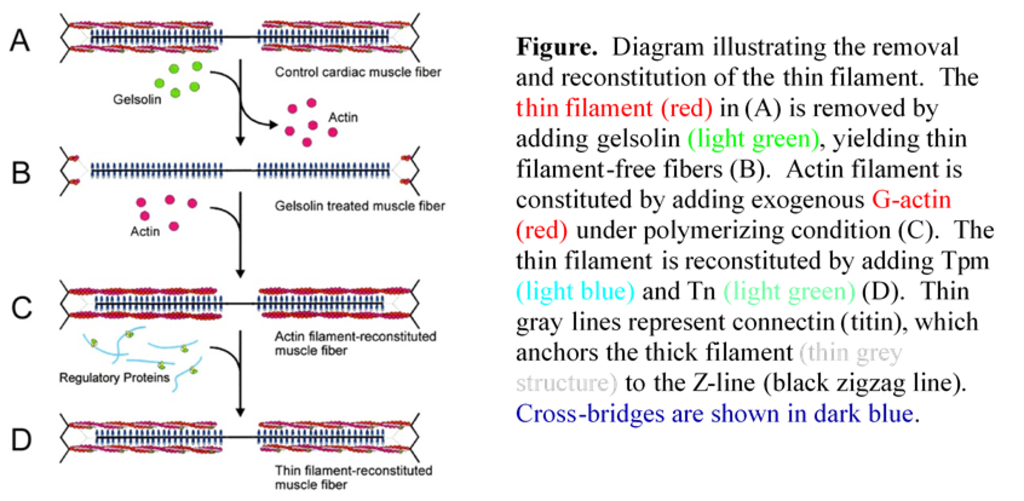
Thin filament removal and reconstruction

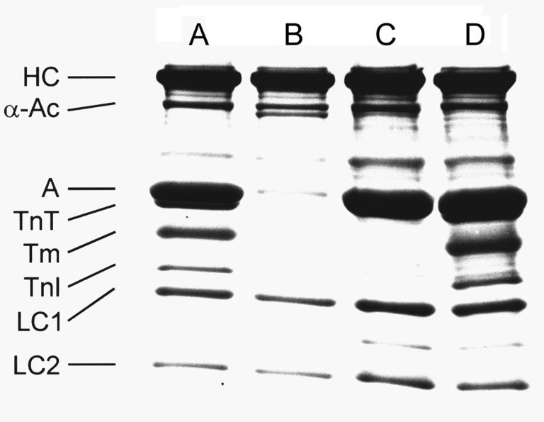
        We have used thin-filament reconstitution technique to study the molecular mechanisms that underlie force generation and the pathogenesis of muscle disease.  As shown in the Figure, this protocol allows us to selectively remove actin-based thin filament of cardiac muscle fibers (myocardium) and to measure force as the filament is reconstituted.  In the first step of this process (A to B), bovine plasma gelsolin is used to dissociate the thin filament.  The actin filament is reconstituted by adding purified G-actin over the course of 28 min (B to C), at which point about 70% the isometric tension is restored.  The thin filament is completely reconstituted by adding the regulatory proteins tropomyosin (Tm, Tpm) and troponin (Tn) in purified form (C to D), and overnight incubation results in full restoration of isometric tension.

        We are using this protocol to study the structure-function relationship of domains in thin-filament proteins, in particular of the domains in actin and Tm.  At each step of reconstitution, the length of the preparation is changed and the concomitant force response is measured.  From the length-force response and the effect of ATP, ADP and phosphate on it, the rate constants and the equilibrium constants of elementary steps of the cross-bridge cycle are deduced, allowing us to characterize the six-state cross-bridge model.  We are finding a steep temperature dependence of tension when Tm and Tn are present, but that this dependence is significantly reduced (by about 50%) in the absence of Tpm and Tn.  These results imply that Tpm and Tn (in the presence of Ca²⁺) have a positive allosteric effect on actin, promoting stereospecific and hydrophobic interactions between actin and myosin molecules. 

       One important use of this reconstituted system is in the analysis of isoform or mutant thin filament proteins (actin, Tpm, Tn).  We have used this method with actin, Tpm and Tm mutants with or without phosphorylation to determine the functional roles of these proteins and their domains.  An example is the significance of N-terminal negative charges of actin in contraction. This method is further used to study mutant proteins that are associated with hypertrophic cardiomyopathy and dilated cardiomyopathy.

Past and present lab members

Postdoctoral Associates

    Li Wang, Yan Zhao, Fan Bai, Xioying Lu, Hideaki Fujita, Wei Ding, Robert N. Cox, PM Gangadhara Swamy, Yankun Peng

Graduate students

    Gang Wang, Julie A. Kapustka Schraeger, Britt Marcussen, Xinping Yue, Chongxia Zhong, Jacqueline Kraus

Undergraduate students with publications

    Karen A Humphries, Thomas W Cornacchia

Research Assistants with publications

    Michael I Schulman, Mary K Bryant, Kristen J Stanton, Heather L Groth, Michael W Wandling, Adam Weiss, Hannah M Caster, Tarek Karam

Visiting scientists

    Yasutake Saeki, Katsuhisa Tawada, Anzel Bahadir, Jing Xi, David W Maughan, Takeyuki Wakabayashi, Howard White, Anders Arner, Antoni Phillipe

Collaborators 

Seminars

Under Construction